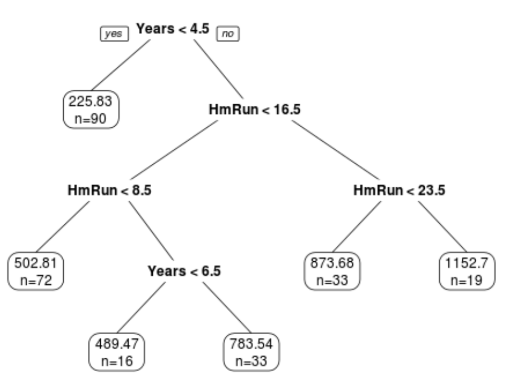
When the relationship between a set of predictor variables and a response variable is highly complex, we often use non-linear methods to model the relationship between them.
One such method is classification and regression trees (often abbreviated CART), which use a set of predictor variables to build decision trees that predict the value of a response variable.

The benefit of decision trees is that they’re easy to interpret and visualize. The downsize is that they tend to suffer from high variance. That is, if we split a dataset into two halves and apply a decision tree to both halves, the results could be quite different.
One way to reduce the variance of decision trees is to use a method known as bagging, which works as follows:
1. Take b bootstrapped samples from the original dataset.
2. Build a decision tree for each bootstrapped sample.
3. Average the predictions of each tree to come up with a final model.
The benefit of this approach is that a bagged model typically offers an improvement in test error rate compared to a single decision tree.
The downside is that the predictions from the collection of bagged trees can be highly correlated if there happens to be a very strong predictor in the dataset. In this case, most or all of the bagged trees will use this predictor for the first split, which will result in trees that are similar to each other and have highly correlated predictions.
Thus, when we average the predictions of each tree to come up with a final bagged model, it’s possible that this model doesn’t actually reduce the variance by much compared to a single decision tree.
One way to get around this issue is to use a method known as random forests.
What Are Random Forests?
Similar to bagging, random forests also take b bootstrapped samples from an original dataset.
However, when building a decision tree for each bootstrapped sample, each time a split in a tree is considered, only a random sample of m predictors is considered as split candidates from the full set of p predictors.
So, here’s the full method that random forests use to build a model:
1. Take b bootstrapped samples from the original dataset.
2. Build a decision tree for each bootstrapped sample.
- When building the tree, each time a split is considered, only a random sample of m predictors is considered as split candidates from the full set of p predictors.
3. Average the predictions of each tree to come up with a final model.
By using this method, the collection of trees in a random forest is decorrelated compared to the trees produced by bagging.
Thus, when we take the average predictions of each tree to come up with a final model it tends to have less variability and results in a lower test error rate compared to a bagged model.
When using random forests, we typically consider m = √p predictors as split candidates each time we split a decision tree.
For example, if we have p = 16 total predictors in a dataset then we typically only consider m = √16 = 4 predictors as potential split candidates at each split.
Technical Note:
It’s interesting to note that if we choose m = p (i.e. we consider all predictors as split candidates at each split) then this is equivalent to simply using bagging.
Out-of-Bag Error Estimation
Similar to bagging, we can calculate the test error of a random forest model by using out-of-bag estimation.
It can be shown that each bootstrapped sample contains about 2/3 of the observations from the original dataset. The remaining 1/3 of the observations not used to fit the tree are referred to as out-of-bag (OOB) observations.
We can predict the value for the ith observation in the original dataset by taking the average prediction from each of the trees in which that observation was OOB.
We can use this approach to make a prediction for all n observations in the original dataset and thus calculate an error rate, which is a valid estimate of the test error.
The benefit of using this approach to estimate the test error is that it’s much quicker than k-fold cross-validation, especially when the dataset is large.
The Pros & Cons of Random Forests
Random forests offer the following benefits:
- In most cases, random forests will offer an improvement in accuracy compared to bagged models and especially compared to single decision trees.
- Random forests are robust to outliers.
- No pre-processing is required to use random forests.
However, random forests come with the following potential drawbacks:
- They’re difficult to interpret.
- They can be computationally intensive (i.e. slow) to build on large datasets.
In practice, data scientists typically use random forests to maximize predictive accuracy so the fact that they’re not easily interpretable is usually not an issue.
