Berkson’s bias is a type of bias that occurs in research when two variables appear to be negatively correlated in sample data, but are actually positively correlated in the overall population.
For example, suppose Tom wants to study the correlation between the quality of burgers and the quality of milkshakes at local restaurants.
He goes out and collects the following data on seven different restaurants:

He creates a scatterplot to visualize the data:
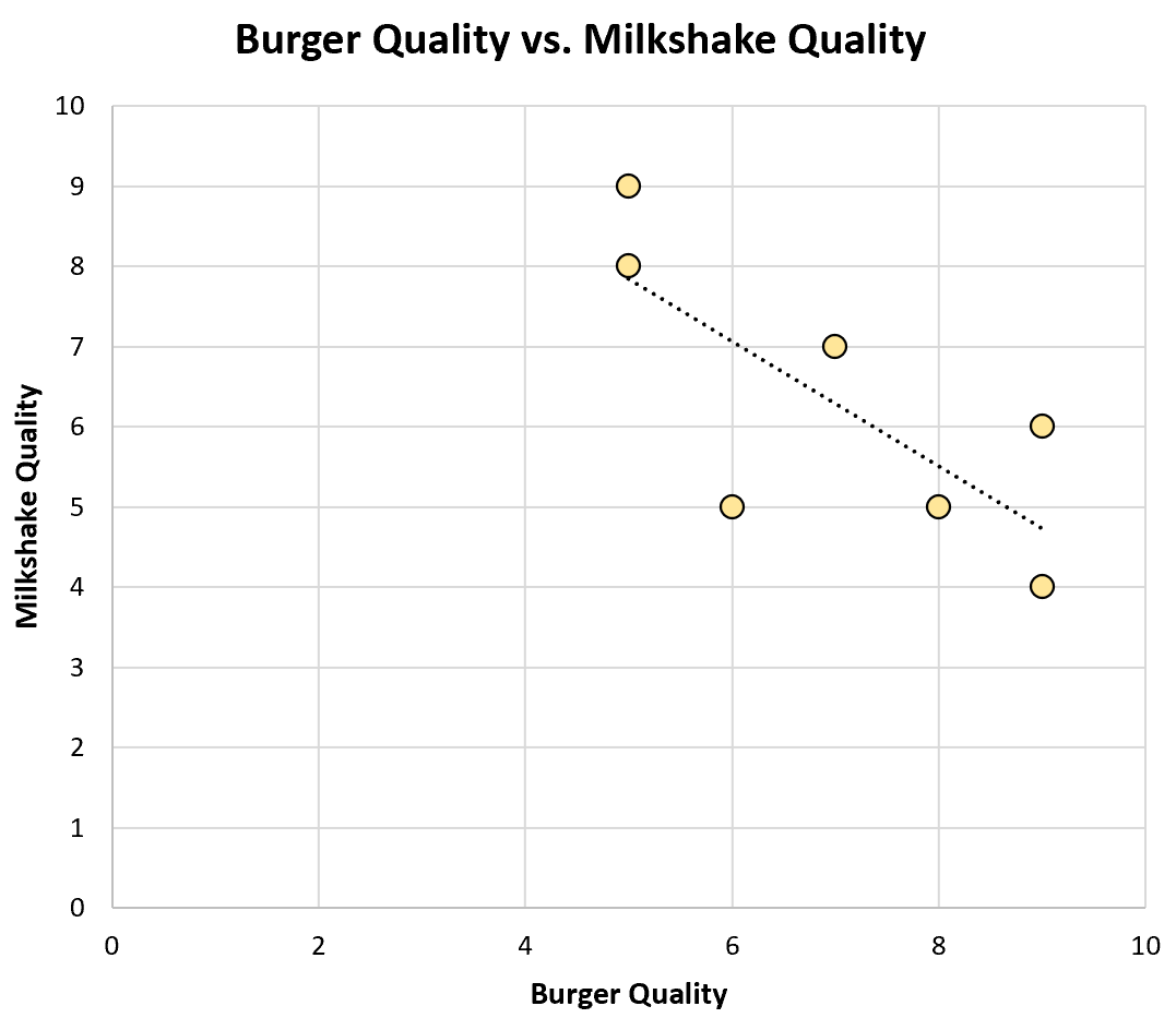
The Pearson correlation coefficient between these two variables is -0.75, which is a strong negative correlation.
This finding is counterintuitive to Tom – He would think that restaurants that make good burgers also make good milkshakes.
However, it turns out that Tom simply skipped over all of the restaurants in town that make both bad burgers and bad milkshakes.
If he had visited these restaurants, he would have collected the following dataset:
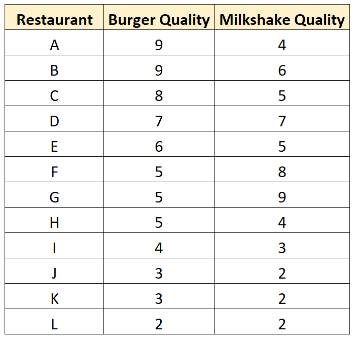
And here’s what a scatterplot for this dataset looks like:
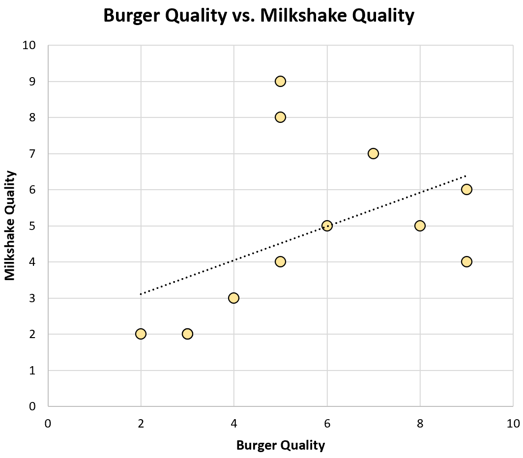
The Pearson correlation coefficient between the two variables turns out to be 0.46, which is a moderately strong positive correlation.
By only looking at a subset of the restaurants in town, Tom incorrectly concluded that there was a negative correlation between burger quality and milkshake quality.
In reality, there turns out to be a positive relationship (as one would expect) between these two variables. This is a classic example of Berkson’s bias.
Check out the following examples for more scenarios where Berkson’s bias occurs in practice.
Example 1: College Admissions
Suppose a college only admits students who have a high enough GPA and high enough ACT score.
It’s well known that these two variables are positively correlated, but it turns out that among the students who decide to go to a particular college, there appears to be a negative correlation between the two.
However, this negative correlation only occurs because the students who have both a high GPA and ACT score may go to an elite university while students who have both a low GPA and ACT score do not get admitted at all.
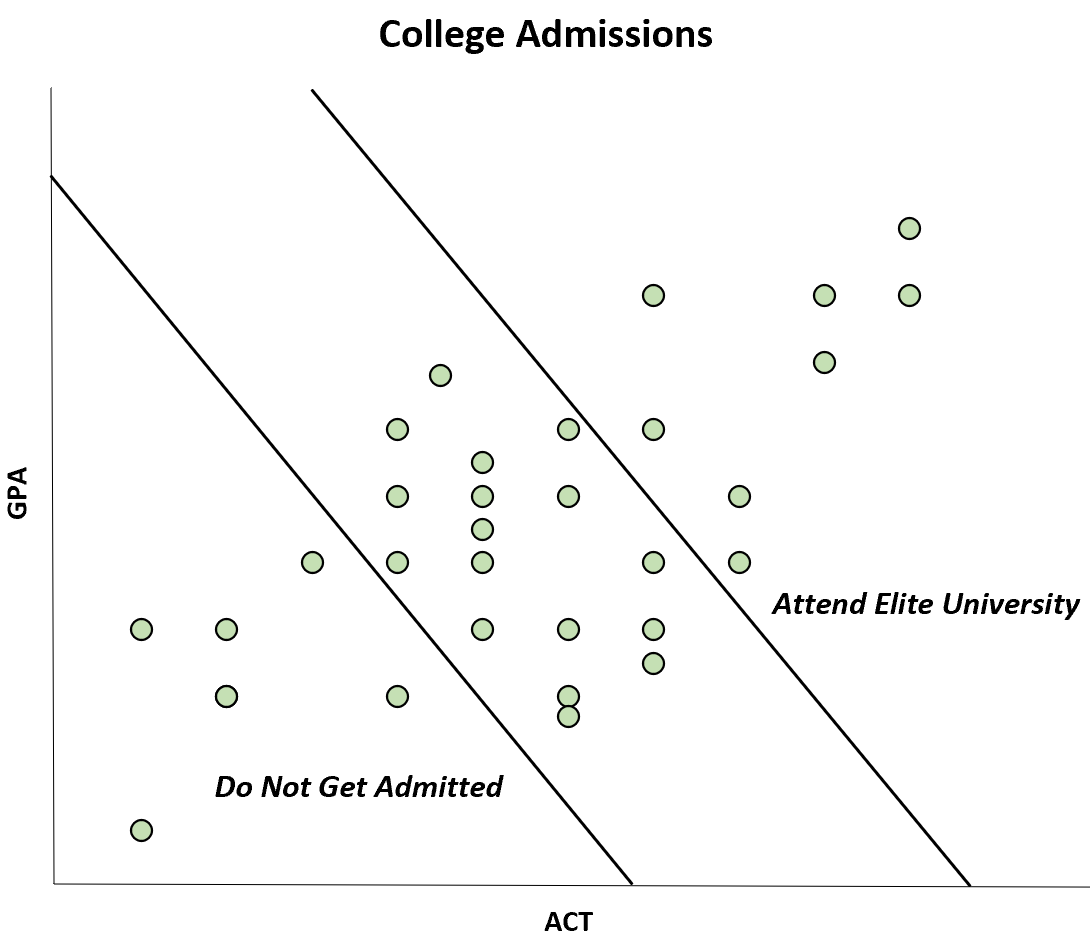
Although the correlation between ACT and GPA is positive in the population, the correlation appears to be negative in the sample. This is a case of Berkson’s bias.
Example 2: Dating Preferences
Many individuals will only date partners who are both attractive and have a good personality.
In the real world, there might be no correlation at all between these two variables, but when narrowing down the dating pool, an individual may completely ignore potential partners who are both unattractive and have a good personality.
Thus, among the potential partners it may seem like there is a negative correlation between these two variables: More attractive people have a worse personality and people with better personalities seem less attractive.
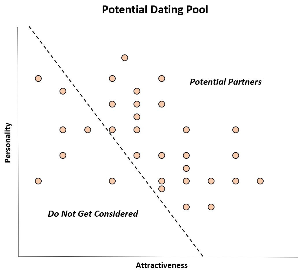
Although there is no correlation between these two variables in the population, there appears to be a negative correlation in the sample of potential partners. This is simply a case of Berkson’s bias.
How to Prevent Berkson’s Bias
The most obvious way to prevent Berkson’s bias in research studies is to collect a simple random sample from a population. That is, make sure that every member of the population of interest has an equal chance of being included in the sample.
For example, if you’re studying the prevalence of diseases in a certain country then you should collect a sample of individuals from around the entire country, not just those individuals who are convenient to reach in hospitals.
By using a simple random sample, researchers can maximize the chances that their sample is representative of the population which means they can generalize their findings from the sample to the overall population with confidence.
