One of the key assumptions of linear regression is that the residuals are distributed with equal variance at each level of the predictor variable. This assumption is known as homoscedasticity.
When this assumption is violated, we say that heteroscedasticity is present in the residuals. When this occurs, the results of the regression become unreliable.
One way to visually detect whether heteroscedasticity is present is to create a plot of the residuals against the fitted values of the regression model.
If the residuals become more spread out at higher values in the plot, this is a tell-tale sign that heteroscedasticity is present.

A formal statistical test we can use to determine if heteroscedasticity is present is the Breusch-Pagan test.
This tutorial provides a brief explanation of the Breusch-Pagan test along with an example.
What is the Breusch-Pagan Test?
The Breusch-Pagan test is used to determine whether or not heteroscedasticity is present in a regression model.
The test uses the following null and alternative hypotheses:
- Null Hypothesis (H0): Homoscedasticity is present (the residuals are distributed with equal variance)
- Alternative Hypothesis (HA): Heteroscedasticity is present (the residuals are not distributed with equal variance)
If the p-value of the test is less than some significance level (i.e. α = .05) then we reject the null hypothesis and conclude that heteroscedasticity is present in the regression model.
We use the following steps to perform a Breusch-Pagan test:
1. Fit the regression model.
2. Calculate the squared residuals of the model.
3. Fit a new regression model, using the squared residuals as the response values.
4. Calculate the Chi-Square test statistic X2 as n*R2new where:
- n: The total number of observations
- R2new: The R-squared of the new regression model that used the squared residuals as the response values
If the p-value that corresponds to this Chi-Square test statistic with p (the number of predictors) degrees of freedom is less than some significance level (i.e. α = .05) then reject the null hypothesis and conclude that heteroscedasticity is present.
Otherwise, fail to reject the null hypothesis. In this case, it’s assumed that homoscedasticity is present.
Note that most statistical software can easily perform the Breusch-Pagan test so you will likely never have to perform these steps by hand, but it’s useful to know what’s going on behind the scenes.
An Example of the Breusch-Pagan Test
Suppose we have the following dataset that contains information for 10 different basketball players:

Using statistical software, we fit the following multiple linear regression model:
rating = 62.47 + 1.12*(points) + 0.88*(assists) – 0.43*(rebounds)
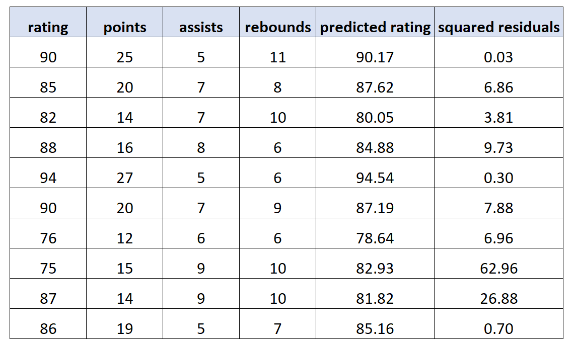
We then use this model to make predictions for the rating of each player and calculated the squared residuals (i.e. the squared difference between the predicted rating and the actual rating):

Next, we fit a new regression model using the squared residuals as the response values and the original predictor variables as the predictor variables once again. We find the following:
- n: 10
- R2new: 0.600395
Thus, our Chi-Square test statistic for the Breusch-Pagan test is n*R2new = 10*.600395 = 6.00395. The degrees of freedom is p = 3 predictor variables.
According to the Chi-Square to P-Value Calculator, the p-value that corresponds to X2 = 6.00395 with 3 degrees of freedom is 0.111418.
Since this p-value is not less than .05, we fail to reject the null hypothesis. Thus, we assume that homoscedasticity is present.
The Breusch-Pagan Test in Practice
The following tutorials provide step-by-step examples of how to perform the Breusch-Pagan test in different statistical programs:
How to Perform a Breusch-Pagan Test in Excel
How to Perform a Breusch-Pagan Test in R
How to Perform a Breusch-Pagan Test in Python
How to Perform a Breusch-Pagan Test in Stata
