Compatible Array Sizes for Basic Operations in MATLAB

Compatible array sizes mean the dimension sizes of the input arrays are either the same, or one of them is scalar, for every dimension. Binary operators and functions operate well with the arrays that have compatible sizes. MATLAB implicitly expands array with compatible sizes to make them the same size during the execution of the element-wise operation or function.

Array Inputs with Compatible Sizes

2-D Array inputs

Let’s understand with some combinations of scalars, vectors, and matrices that have compatible sizes:

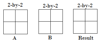
• Two array inputs are exactly of the same size.

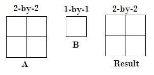
• One array input is a scalar.

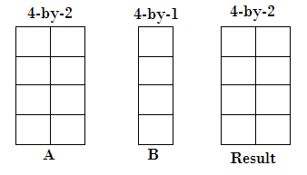
• One input is a matrix, and another is a column vector with a similar number of rows.

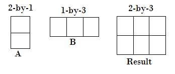
• One input is a column vector, and another is a row vector.

Multi-dimensional Array Input

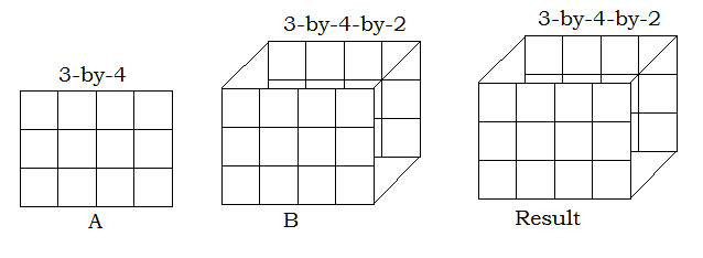
• One input is a matrix, and the other is a 3-D array with the same number of rows and columns.

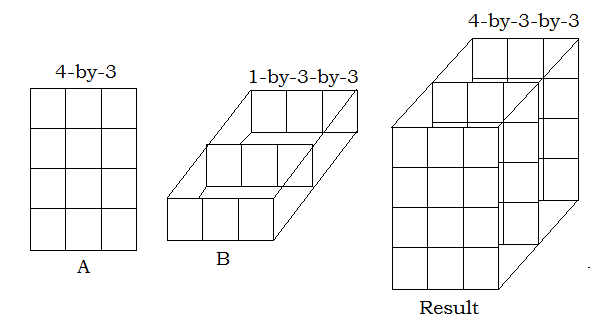
• One input is a matrix, and the other is a 3-D array. The dimensions of all inputs are all either the same, or one of the inputs is 1-D.

Empty Array input

Empty arrays are the arrays with no elements and dimension size of zero. The rules for empty arrays and non-empty arrays are the same, and the size of the dimension that is not equal to 1 determines the size of the output.

Example:

Output:

>> a.*b    ans =      3x3x0 empty double array  

MATLAB implicitly expands arrays with compatible sizes, but incompatible sizes cannot be implicitly expanded to be the same size.

• One of the input dimension sizes is neither equal nor one.

Example:

Output:

>> a+b  Matrix dimensions must agree.  >> a-b  Matrix dimensions must agree.  >> a.*b  Matrix dimensions must agree.  

• Two non-scalar row vectors with non-equal lengths.

Example:

Output:

>> a+b  Matrix dimensions must agree.    >> a-b  Matrix dimensions must agree.    >> a.*b  Matrix dimensions must agree  

Row and Column Vector Compatibility

Row and column vectors always have compatible sizes, even with different sizes and lengths. And performing arithmetic operations on these vectors creates a matrix.

Example:

Output:

   >>% adding two row and column vectors  >> a + b  ans =      1.9058    1.9058    1.9058      1.1270    1.1270    1.1270      1.9134    1.9134    1.9134      1.6324    1.6324    1.6324    >>% subtraction of two row and column vectors  >> a - b  ans =      0.0942    0.0942    0.0942      0.8730    0.8730    0.8730      0.0866    0.0866    0.0866      0.3676    0.3676    0.3676    >>% array multiplication of two row and column vectors  >> a.*b  ans =      0.9058    0.9058    0.9058      0.1270    0.1270    0.1270      0.9134    0.9134    0.9134      0.6324    0.6324    0.6324