A crosstab is a table that summarizes the relationship between two categorical variables.
The following step-by-step example explains how to create a crosstab in Excel.
Step 1: Enter the Data
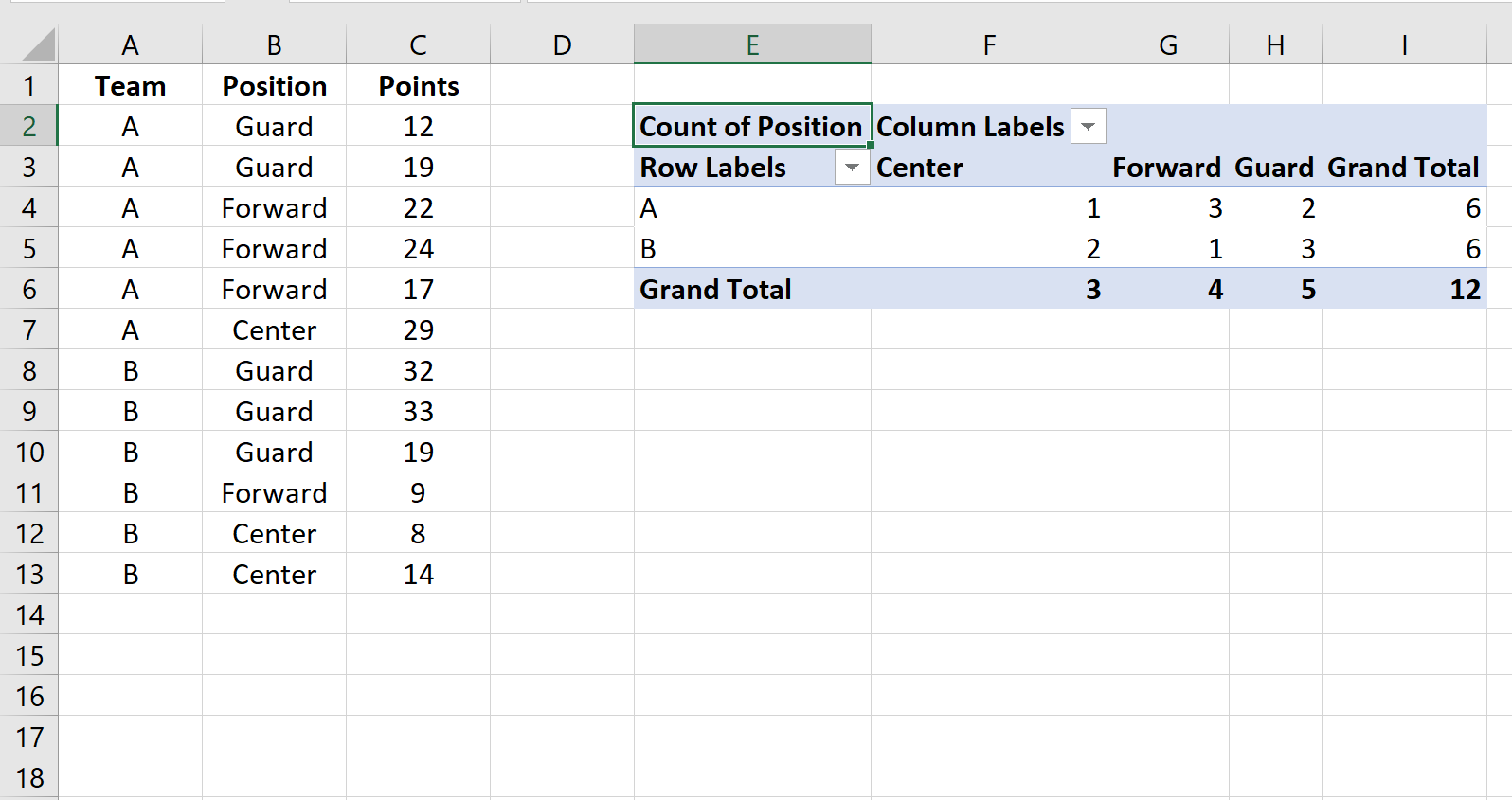
First, let’s enter the following dataset into Excel:

Step 2: Create the Crosstab
Next, click the Insert tab along the top ribbon and then click the PivotTable button.

In the new window that appears, select the range that contains the data as the Table/Range and choose any cell you’d like in the Existing Worksheet to place the crosstab. We’ll choose cell E2:

Step 3: Populate the Crosstab with Values
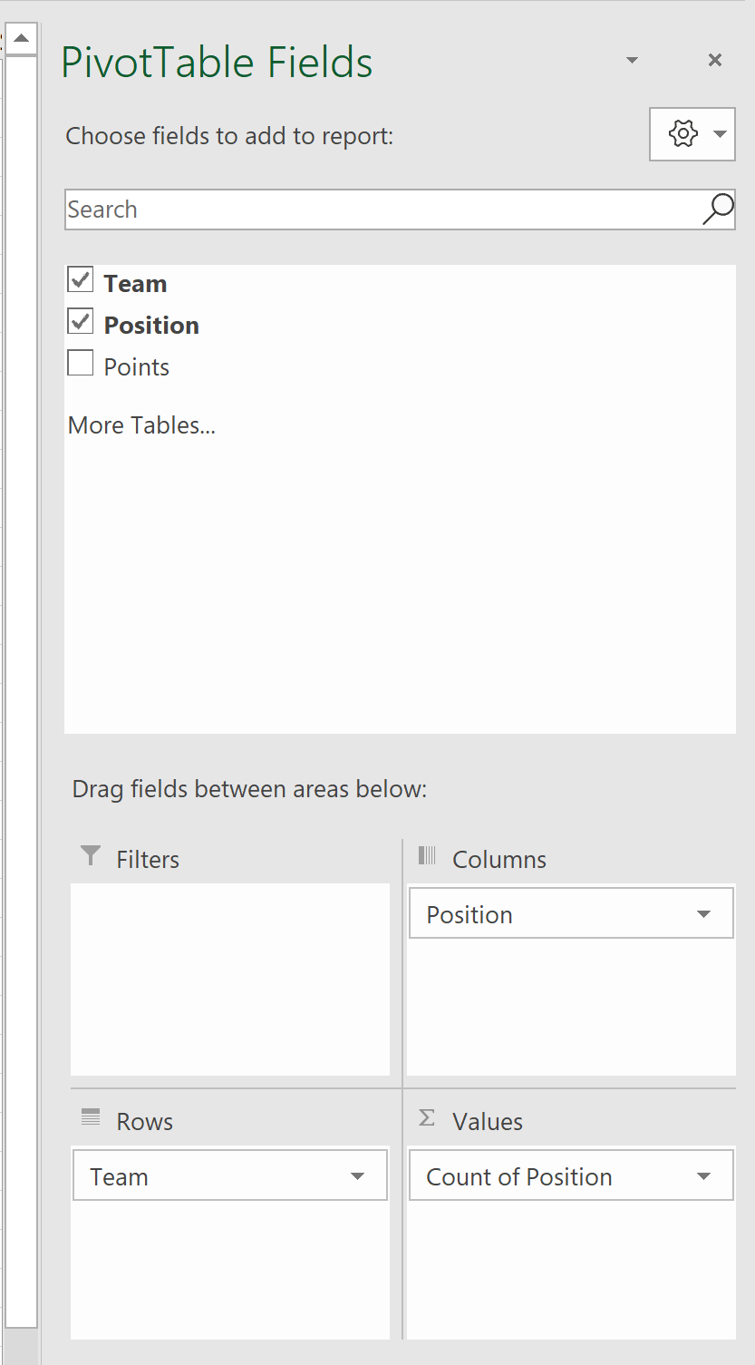
Once you click OK, a new window on the right side of the screen will appear.
Drag the Team variable to the Rows area, the Position variable to the Columns area, then the Position variable again to the Values area as follows:

Once you do so, the following crosstab will appear in the cell that you specified:

Step 4: Interpret the Crosstab
Here’s how to interpret the values in the crosstab:
Row Totals:
- A total of 6 players are on team A
- A total of 6 players are on team B
Column Totals:
- A total of 3 players have a position of Center
- A total of 4 players have a position of Forward
- A total of 5 players have a position of Guard
Individual Cells:
- 1 player has a position of Center on team A
- 3 players have a position of Forward on team A
- 2 players have a position of Guard on team A
- 2 players have a position of Center on team B
- 1 player has a position of Forward on team B
- 3 players have a position of Guard on team B
Additional Resources
The following tutorials offer additional information on how to calculate frequencies in Excel:
How to Calculate Relative Frequency in Excel
How to Calculate Cumulative Frequency in Excel
How to Create a Frequency Polygon in Excel
