How to Perform Cubic Regression in Python

---

Cubic regression is a type of regression we can use to quantify the relationship between a predictor variable and a response variable when the relationship between the variables is non-linear.

This tutorial explains how to perform cubic regression in Python.

Example: Cubic Regression in Python

Suppose we have the following pandas DataFrame that contains two variables (x and y):

import pandas as pd

#create DataFrame
df = pd.DataFrame({'x': [6, 9, 12, 16, 22, 28, 33, 40, 47, 51, 55, 60],
                   'y': [14, 28, 50, 64, 67, 57, 55, 57, 68, 74, 88, 110]})

#view DataFrame
print(df)

     x    y
0    6   14
1    9   28
2   12   50
3   16   64
4   22   67
5   28   57
6   33   55
7   40   57
8   47   68
9   51   74
10  55   88
11  60  110

If we make a simple scatterplot of this data we can see that the relationship between the two variables is non-linear:

import matplotlib.pyplot as plt

#create scatterplot
plt.scatter(df.x, df.y)

As the value for x increases, y increases up to a certain point, then decreases, then increases once more.

This pattern with two “curves” in the plot is an indication of a cubic relationship between the two variables.

This means a cubic regression model is a good candidate for quantifying the relationship between the two variables.

To perform cubic regression, we can fit a polynomial regression model with a degree of 3 using the numpy.polyfit() function:

import numpy as np

#fit cubic regression model
model = np.poly1d(np.polyfit(df.x, df.y, 3))

#add fitted cubic regression line to scatterplot
polyline = np.linspace(1, 60, 50)
plt.scatter(df.x, df.y)
plt.plot(polyline, model(polyline))

#add axis labels
plt.xlabel('x')
plt.ylabel('y')

#display plot
plt.show()

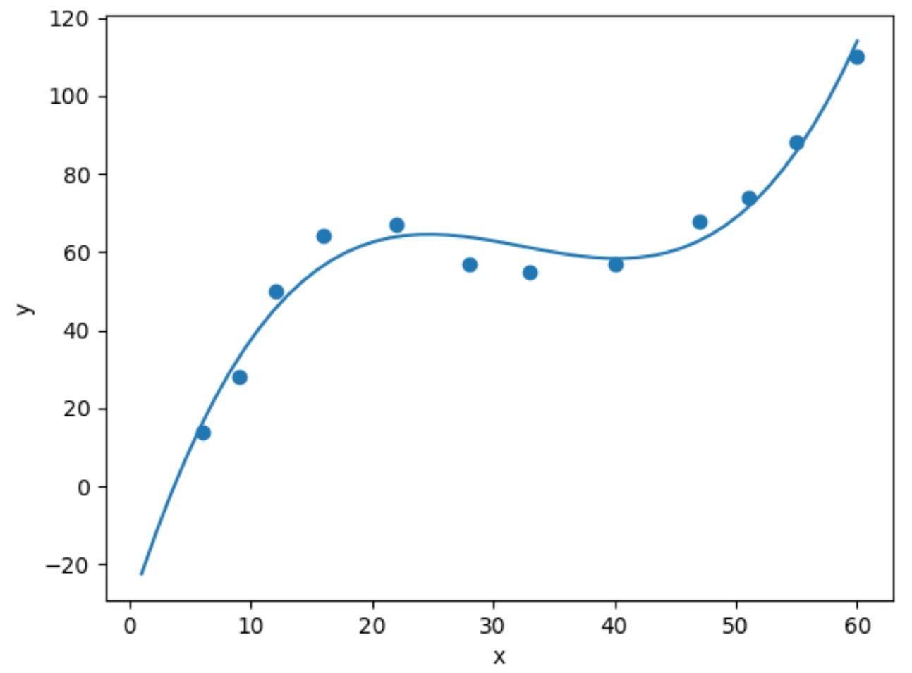
We can obtain the fitted cubic regression equation by printing the model coefficients:

print(model)

          3          2
0.003302 x - 0.3214 x + 9.832 x - 32.01

The fitted cubic regression equation is:

y = 0.003302(x)³ – 0.3214(x)² + 9.832x – 30.01

We can use this equation to calculate the expected value for y based on the value for x.

For example, if x is equal to 30 then the expected value for y is 64.844:

y = 0.003302(30)³ – 0.3214(30)² + 9.832(30) – 30.01 = 64.844

We can also write a short function to obtain the R-squared of the model, which is the proportion of the variance in the response variable that can be explained by the predictor variables.

#define function to calculate r-squared
def polyfit(x, y, degree):
    results = {}
    coeffs = np.polyfit(x, y, degree)
    p = np.poly1d(coeffs)
    #calculate r-squared
    yhat = p(x)
    ybar = np.sum(y)/len(y)
    ssreg = np.sum((yhat-ybar)**2)
    sstot = np.sum((y - ybar)**2)
    results['r_squared'] = ssreg / sstot

    return results

#find r-squared of polynomial model with degree = 3
polyfit(df.x, df.y, 3)

{'r_squared': 0.9632469890057967}

In this example, the R-squared of the model is 0.9632.

This means that 96.32% of the variation in the response variable can be explained by the predictor variable.

Since this value is so high, it tells us that the cubic regression model does a good job of quantifying the relationship between the two variables.

Related: What is a Good R-squared Value?

Additional Resources

The following tutorials explain how to perform other common tasks in Python:

How to Perform Simple Linear Regression in Python
How to Perform Quadratic Regression in Python
How to Perform Polynomial Regression in Python