Excel: How to Group Values in Pivot Table by Range

---

The following step-by-step example shows how to group values in a pivot table in Excel by range.

Step 1: Enter the Data

First, let’s enter the following data about 15 different stores:

Step 2: Create Pivot Table

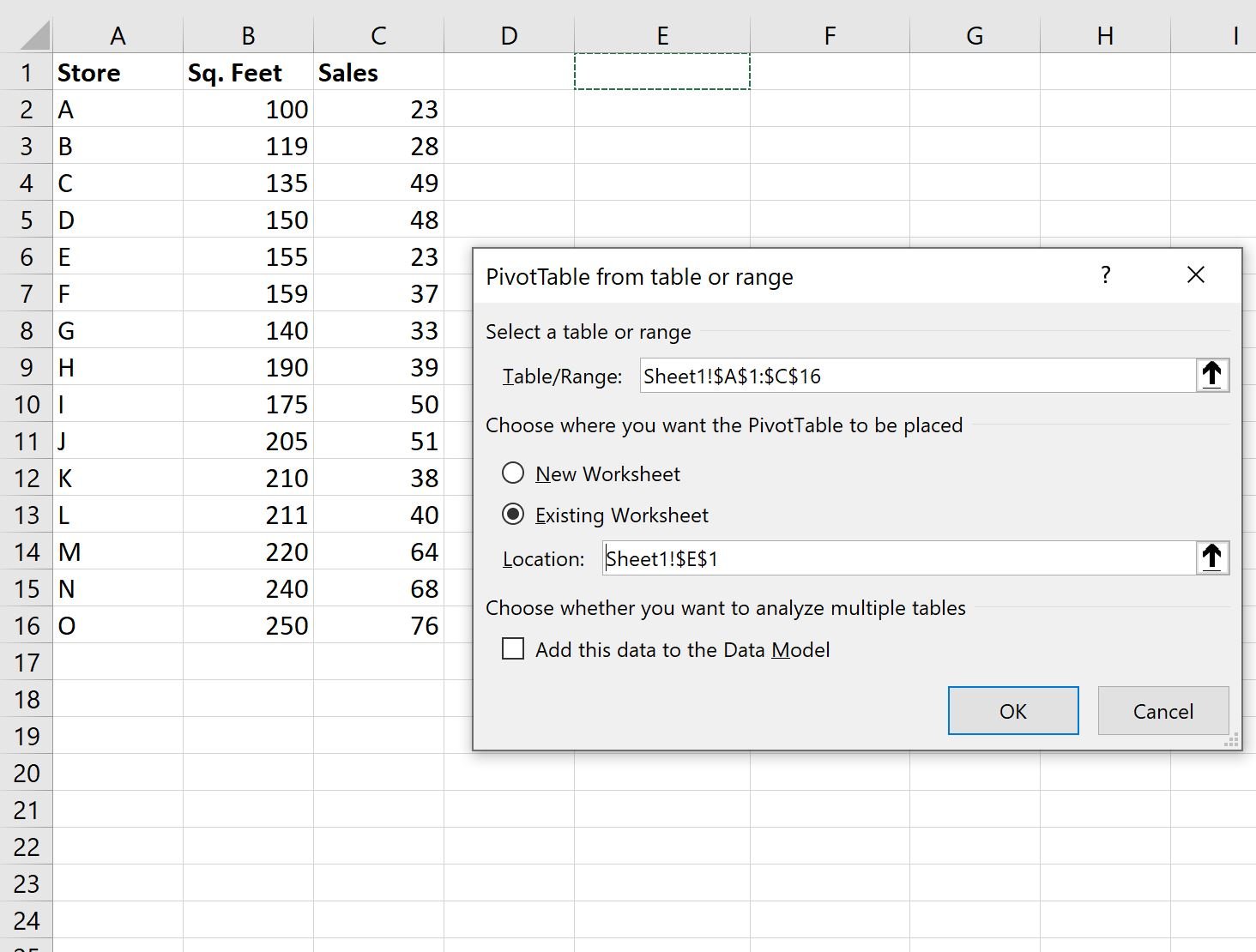
To create a pivot table from this data, click the Insert tab along the top ribbon and then click the PivotTable icon:

In the new window that appears, choose A1:C16 as the range and choose to place the pivot table in cell E1 of the existing worksheet:

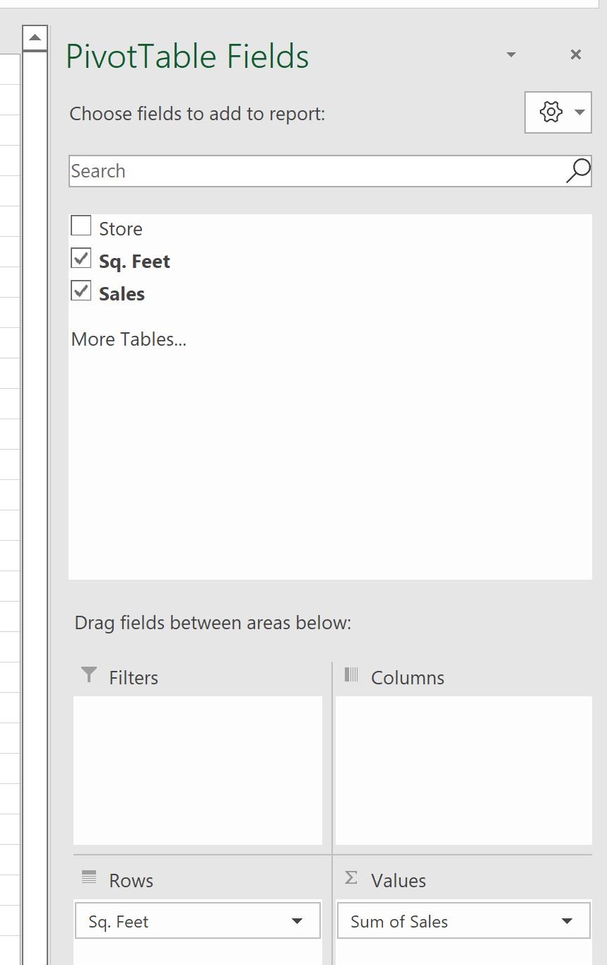
Once you click OK, a new PivotTable Fields panel will appear on the right side of the screen.

Drag the Sq. Feet field to the Rows box and drag the Sales field to the Values box:

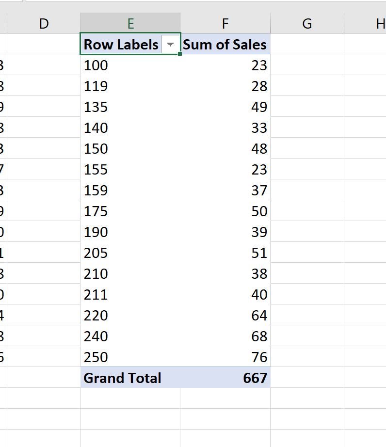
The pivot table will automatically be populated with the following values:

 

Step 3: Group Pivot Table Values by Range

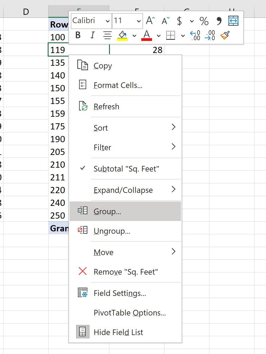
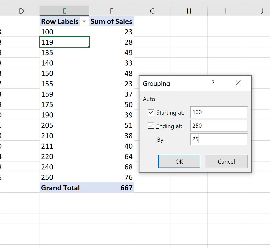
To group the square footage values by range, right click on any value in the first column of the pivot table, then click Group in the dropdown menu:

In the Grouping window that appears, choose to group values starting at 100, ending at 250, by 25:

Once you click OK, the square footage values in the pivot table will automatically be grouped from 100 to 250, in ranges of length 25:

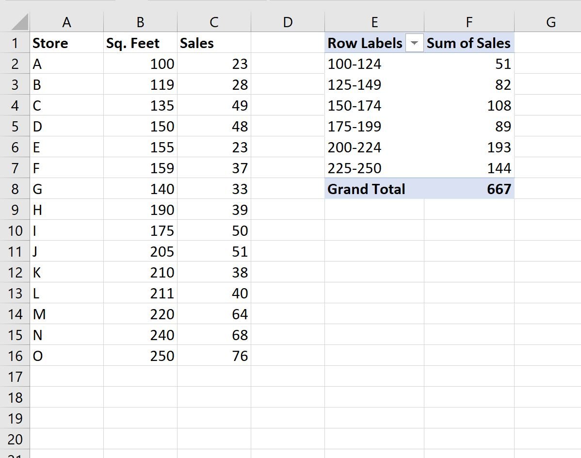
Here’s how to interpret the values in the pivot table:

• The sum of the sales for stores with square footage between 100 and 124 is 51.
• The sum of the sales for stores with square footage between 125 and 149 is 82.
• The sum of the sales for stores with square footage between 150 and 174 is 108.

And so on.

For this example we grouped the values using a range of 25, but feel free to use whatever range you’d like depending on your data.

Additional Resources

The following tutorials explain how to perform other common tasks in Excel:

How to Create Tables in Excel
How to Create a Contingency Table in Excel
How to Group by Month and Year in Pivot Table in Excel