This step-by-step tutorial explains how to create the following progress bars in Excel:
Step 1: Enter the Data
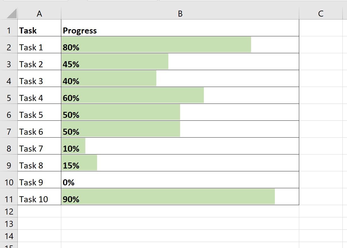
First, let’s enter some data that shows the progress percentage for 10 different tasks:

Step 2: Add the Progress Bars
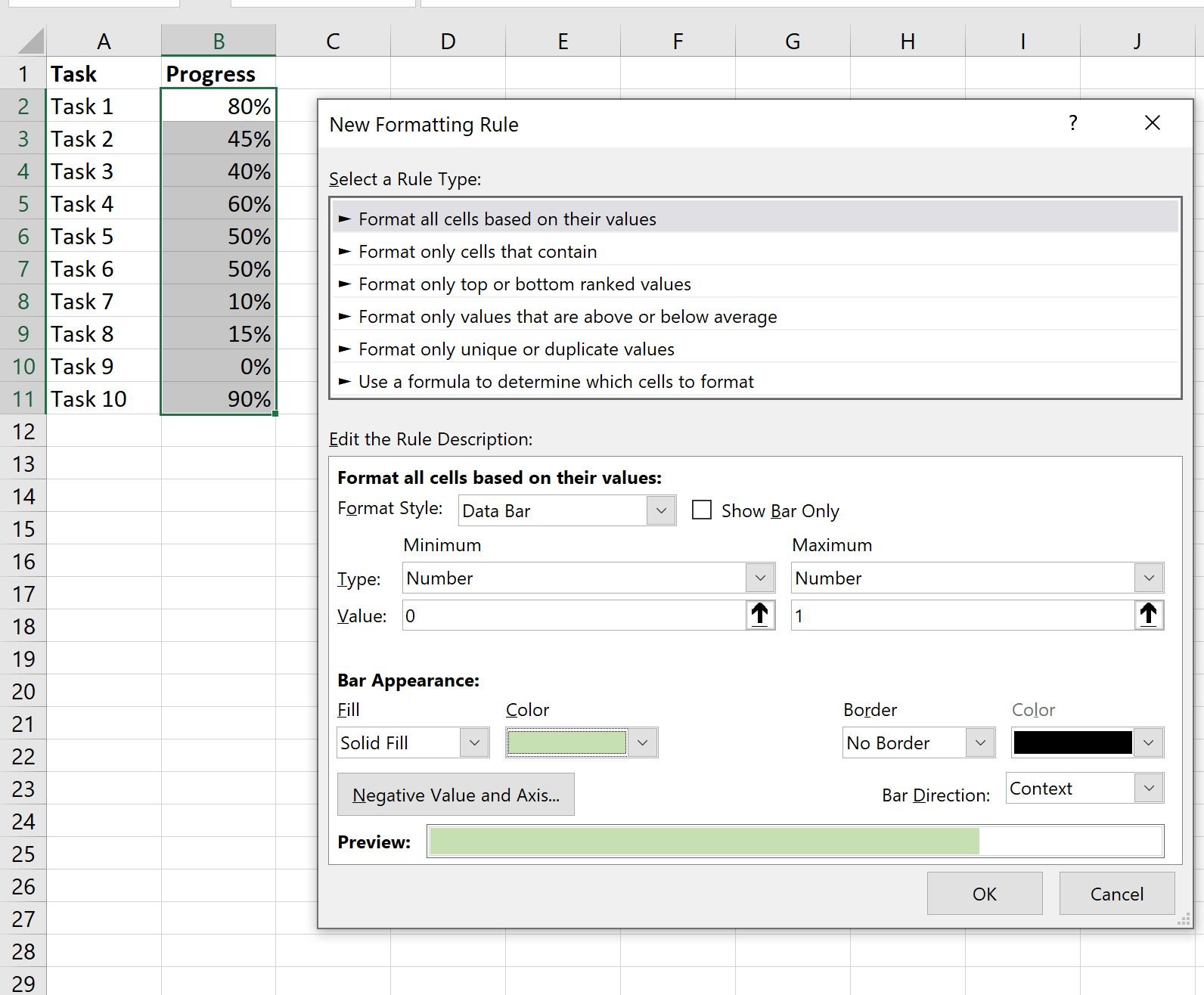
Next, highlight the cell range B2:B11 that contains the progress percentages, then click the Conditional Formatting icon on the Home tab, then click Data Bars, then click More Rules:

A new window appears that allows you to format the data bars.
For Minimum, change the Type to Number and the Value to 0.
For Maximum, change the Type to Number and the Value to 1.
Then choose any color you’d like for the bars. We’ll choose light green:
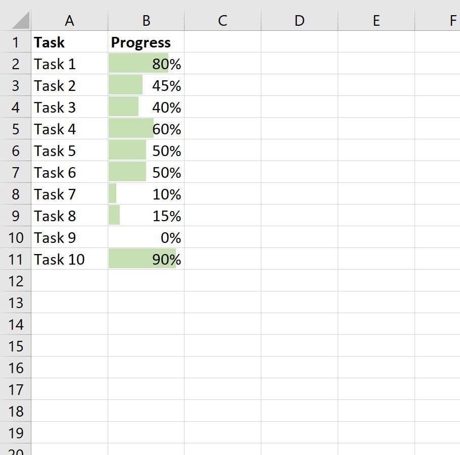
Once you click OK, a progress bar will appear in each cell in column B:
Step 3: Format the Progress Bars
Lastly, we can stretch out the column width and row width in our Excel spreadsheet so that the progress bars become larger and easier to read.
We can also add a border around the cells and align the text for the percentages to be on the left side of the cells:
Note that if you update any of the percentages, the length of the progress bar will automatically change.
For example, suppose we change the last progress percentage to 22%:

Notice that the progress bar automatically shortened to reflect this new percentage.
Additional Resources
The following tutorials explain how to perform other common tasks in Excel:
How to Create a Gantt Chart in Excel
How to Create a Double Doughnut Chart in Excel
How to Create a Statistical Process Control Chart in Excel