You can use the following basic syntax to replace #N/A values in Excel with either zeros or blanks:
#replace #N/A with zero
=IFERROR(FORMULA, "0")

#replace #N/A with blank
=IFERROR(FORMULA, "")
The following example shows how to use this syntax in practice to replace #N/A values from a VLOOKUP with zero or blanks.
Related: How to Replace Blank Cells with Zero in Excel
Example: Replace #N/A Values in Excel
Suppose we have the following dataset in Excel:

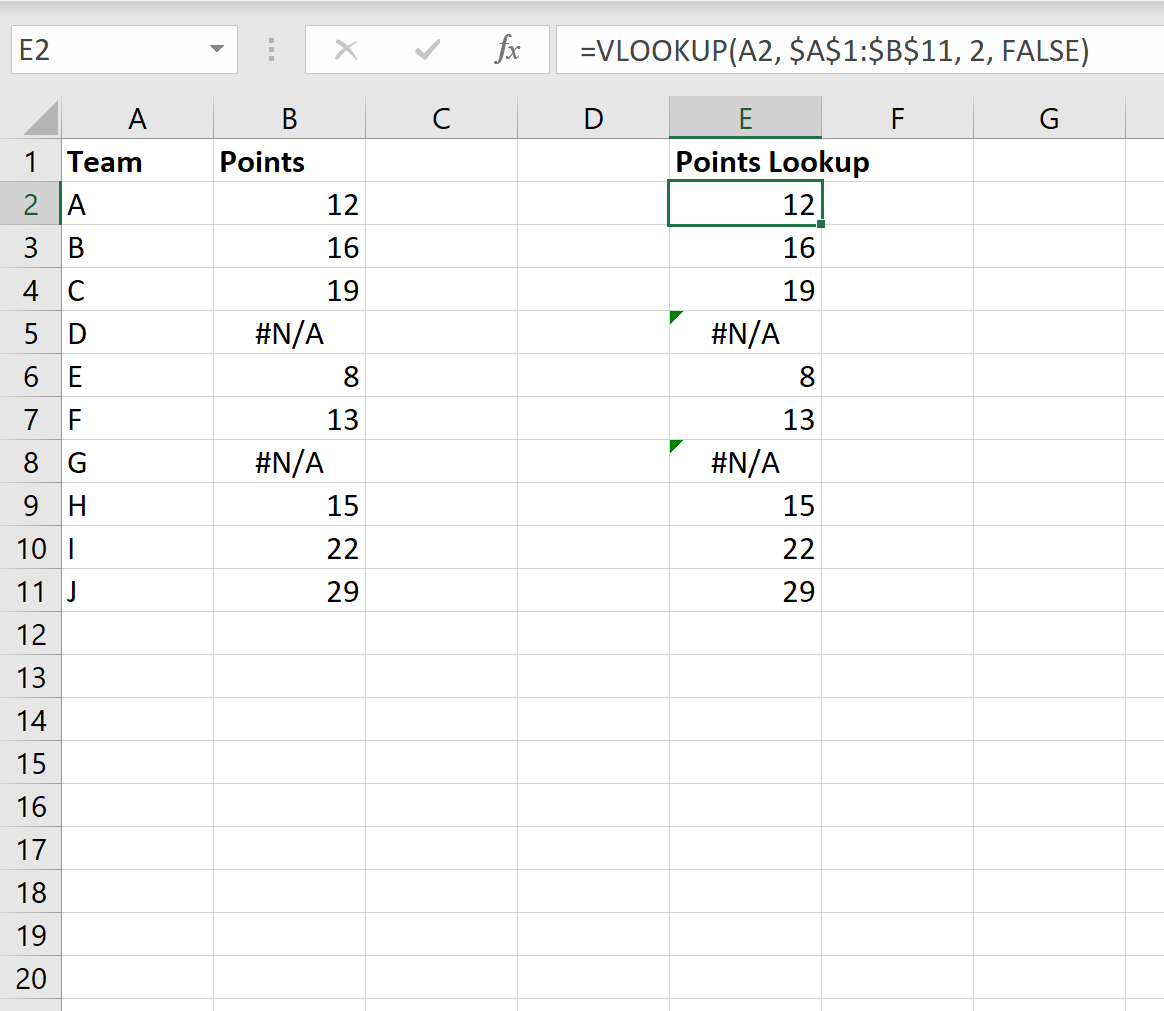
And suppose we use the VLOOKUP() function to look up points based on team name:

Notice that some of the values returned in the VLOOKUP() are #N/A values.
We can turn these values into zeros by using the IFERROR() function as follows:
#replace #N/A with zero
=IFERROR(VLOOKUP(A2, $A$1:$B$11, 2, FALSE), "0")
The following screenshot shows how to use this function in practice:

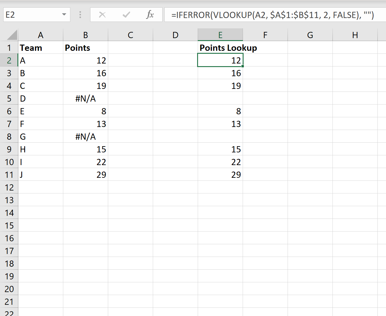
Alternatively, we can turn the #N/A values into blanks using the IFERROR() function as follows:
#replace #N/A with blank
=IFERROR(VLOOKUP(A2, $A$1:$B$11, 2, FALSE), "")
The following screenshot shows how to use this function in practice:

Notice that each value that was previously #N/A is now blank.
Using the IFERROR() function, we can replace #N/A values with any value that we’d like.
In the previous examples, we simply chose to replace #N/A values with zeros or blanks because these are the most common replacement values used in practice.
Additional Resources
How to Perform a Percentile IF Function in Excel
How to Perform a Median IF Function in Excel
