How to Use LOGEST Function in Excel (With Example)

---

You can use the LOGEST function in Excel to calculate the formula of an exponential curve that fits your data.

The equation of the curve will take on the following form:

y = b * m^x

This function uses the following basic syntax:

=LOGEST(known_y's, [known_x's], [const], [stats])

where:

• known_y’s: An array of known y-values
• known_x’s: An array of known x-values
• const: Optional argument. If TRUE, the constant b is treated normally. If FALSE, the constant b is set to 1.
• stats: Optional argument. If TRUE, additional regression statistics are returned. If FALSE, additional regression statistics are not returned.

The following step-by-step example shows how to use this function in practice.

Step 1: Enter the Data

First, let’s enter the following dataset in Excel:

Step 2: Visualize the Data

Next, let’s create a quick scatter plot of x vs. y to verify that the data actually follow an exponential curve:

We can see that the data do indeed follow an exponential curve.

Step 3: Use LOGEST to Find the Exponential Curve Formula

Next, we can type the following formula into any cell to calculate the exponential curve formula:

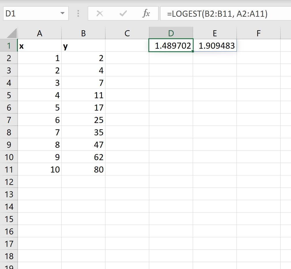
=LOGEST(B2:B11, A2:A11)

The following screenshot shows how to use this formula in practice:

The first value in the output represents the value for m and the second value in the output represents the value for b in the equation:

y = b * m^x

Thus, we would write this exponential curve formula as:

y = 1.909483 * 1.489702^x

We could then use this formula to predict the values of y based on the value of x.

For example, if x has a value of 8 then we would predict that y has a value of 46.31:

y = 1.909483 * 1.489702⁸ = 46.31

Step 4 (Optional): Display Additional Regression Statistics

We can set the value for the stats argument in the LOGEST function equal to TRUE to display additional regression statistics for the fitted regression equation:

Here’s how to interpret each value in the output:

• The standard error for m is .02206.
• The standard error for b is .136879.
• The R² for the model is .97608.
• The standard error for y is .200371.
• The F-statistic is 326.4436.
• The degrees of freedom is 8.
• The regression sum of squares is 13.10617.
• The residual sum of squares is .321187.

In general, the most interesting metric in these additional statistics is the R² value, which represents the proportion of the variance in the response variable that can be explained the predictor variable.

The value for R² can range from 0 to 1.

Since the R² for this particular model is close to 1, it tells us that the predictor variable x does a good job of predicting the value of the response variable y.

Related: What is a Good R-squared Value?

Additional Resources

The following tutorials explain how to perform other common operations in Excel:

How to Use DEVSQ in Excel
How to Use SUMSQ in Excel
How to Perform Nonlinear Regression in Excel