How to Perform Multiple Linear Regression in SPSS

---

Multiple linear regression is a method we can use to understand the relationship between two or more explanatory variables and a response variable.

This tutorial explains how to perform multiple linear regression in SPSS.

Example: Multiple Linear Regression in SPSS

Suppose we want to know if the number of hours spent studying and the number of prep exams taken affects the score that a student receives on a certain exam. To explore this, we can perform multiple linear regression using the following variables:

Explanatory variables:

• Hours studied
• Prep exams taken

Response variable:

• Exam score

Use the following steps to perform this multiple linear regression in SPSS.

Step 1: Enter the data.

Enter the following data for the number of hours studied, prep exams taken, and exam score received for 20 students:

Step 2: Perform multiple linear regression.

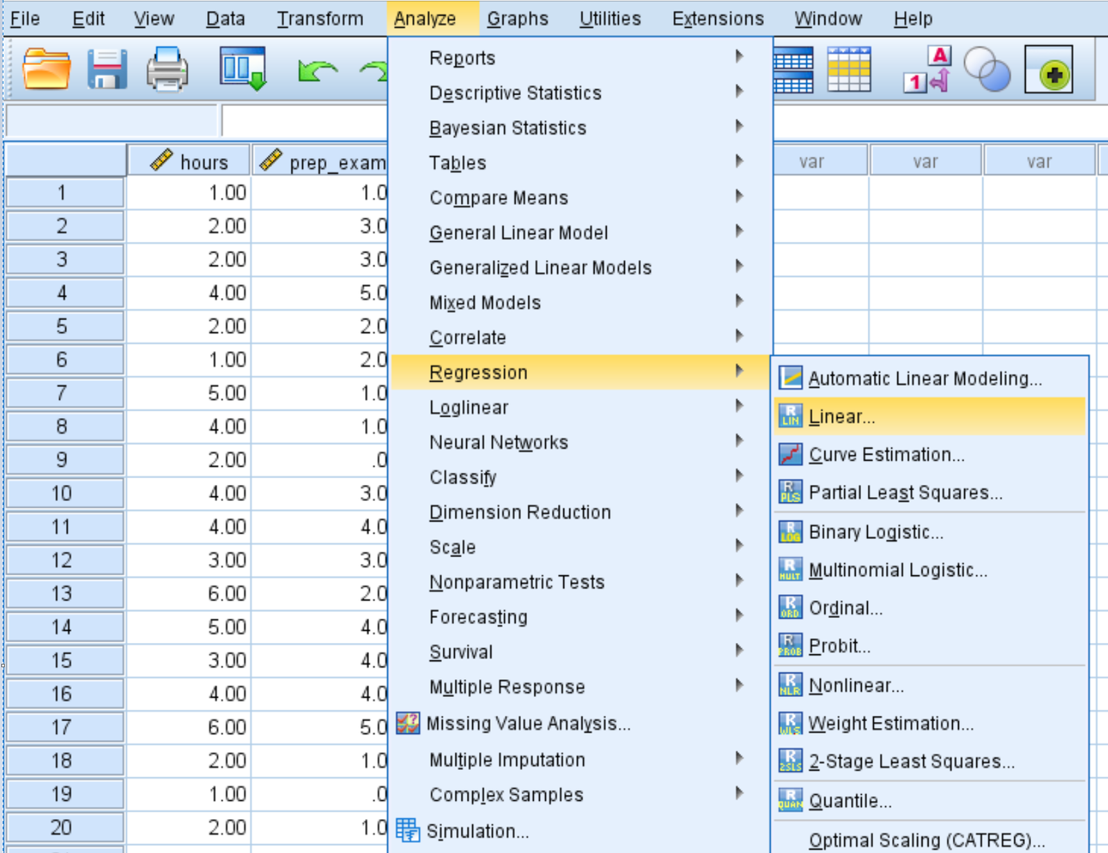
Click the Analyze tab, then Regression, then Linear:

Drag the variable score into the box labelled Dependent. Drag the variables hours and prep_exams into the box labelled Independent(s). Then click OK.

Step 3: Interpret the output.

Once you click OK, the results of the multiple linear regression will appear in a new window.

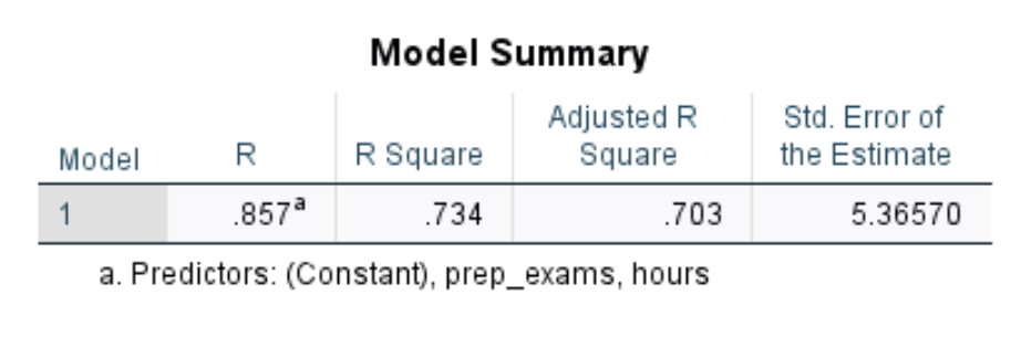
The first table we’re interested in is titled Model Summary:

Here is how to interpret the most relevant numbers in this table:

• R Square: This is the proportion of the variance in the response variable that can be explained by the explanatory variables. In this example, 73.4% of the variation in exam scores can be explained by hours studied and number of prep exams taken.
• Std. Error of the Estimate: The standard error is the average distance that the observed values fall from the regression line. In this example, the observed values fall an average of 5.3657 units from the regression line.

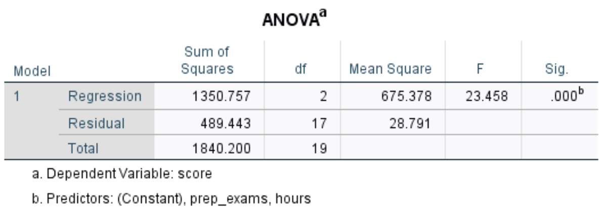
The next table we’re interested in is titled ANOVA:

Here is how to interpret the most relevant numbers in this table:

• F: This is the overall F statistic for the regression model, calculated as Mean Square Regression / Mean Square Residual.
• Sig: This is the p-value associated with the overall F statistic. It tells us whether or not the regression model as a whole is statistically significant. In other words, it tells us if the two explanatory variables combined have a statistically significant association with the response variable. In this case the p-value is equal to 0.000, which indicates that the explanatory variables hours studied and prep exams taken have a statistically significant association with exam score.

The next table we’re interested in is titled Coefficients:

Here is how to interpret the most relevant numbers in this table:

• Unstandardized B (Constant): This tells us the average value of the response variable when both predictor variables are zero. In this example, the average exam score is 67.674 when hours studied and prep exams taken are both equal to zero.
• Unstandardized B (hours): This tells us the average change in exam score associated with a one unit increase in hours studied, assuming number of prep exams taken is held constant. In this case, each additional hour spent studying is associated with an increase of 5.556 points in exam score, assuming the number of prep exams taken is held constant.
• Unstandardized B (prep_exams): This tells us the average change in exam score associated with a one unit increase in prep exams taken, assuming number of hours studied is held constant. In this case, each additional prep exam taken is associated with a decrease of .602 points in exam score, assuming the number of hours studied is held constant.
• Sig. (hours): This is the p-value for the explanatory variable hours. Since this value (.000) is less than .05, we can conclude that hours studied has a statistically significant association with exam score.
• Sig. (prep_exams): This is the p-value for the explanatory variable prep_exams. Since this value (.519) is not less than .05, we cannot conclude that number of prep exams taken has a statistically significant association with exam score.

Lastly, we can form a regression equation using the values shown in the table for constant, hours, and prep_exams. In this case, the equation would be:

Estimated exam score = 67.674 + 5.556*(hours) – .602*(prep_exams)

We can use this equation to find the estimated exam score for a student, based on the number of hours they studied and the number of prep exams they took. For example, a student that studies for 3 hours and takes 2 prep exams is expected to receive an exam score of 83.1:

Estimated exam score = 67.674 + 5.556*(3) – .602*(2) = 83.1

Note: Since the explanatory variable prep exams was not found to be statistically significant, we may decide to remove it from the model and instead perform simple linear regression using hours studied as the only explanatory variable.