A probability mass function, often abbreviated PMF, tells us the probability that a discrete random variable takes on a certain value.
For example, suppose we roll a dice one time. If we let x denote the number that the dice lands on, then the probability that the x is equal to different values can be described as follows:
- P(X=1): 1/6
- P(X=2): 1/6
- P(X=3): 1/6
- P(X=4): 1/6
- P(X=5): 1/6
- P(X=6): 1/6
There is an equal chance that the dice could land on any number between 1 and 6.
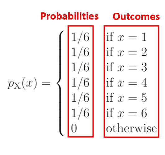
Here’s how we would write these probabilities as a probability mass function:

The left side of the diagram shows the probability associated with the outcomes on the right side:

One characteristic of a probability mass function is that all of the probabilities must add up to 1. You’ll notice that this PMF satisfies that condition:
Sum of probabilities = 1/6 + 1/6 + 1/6 + 1/6 + 1/6 + 1/6 = 1.
The support of a probability mass function refers to the set of values that the discrete random variable can take. In this example, the support would be {1, 2, 3, 4, 5, 6} since the value of the dice can take on any of these values.
Outside of the support, the value for the PMF is equal to zero. For example, the probability that the dice lands on “0” or “7” or “8” is equal to zero since none of these numbers are included in the support.
Probability Mass Functions in Practice
The two most common examples of probability mass functions in practice are for the Binomial distribution and the Poisson distribution.
Binomial Distribution
If a random variable X follows a Binomial distribution, then the probability that X = k successes can be found by the following formula:
P(X=k) = nCk * pk * (1-p)n-k
where:
- n: number of trials
- k: number of successes
- p: probability of success on a given trial
- nCk: the number of ways to obtain k successes in n trials
For example, suppose we flip a coin 3 times. We can use the formula above to determine the probability of obtaining 0, 1, 2, and 3 heads during these 3 flips:
- P(X=0) = 3C0 * .50 * (1-.5)3-0 = 1 * 1 * (.5)3 = 0.125
- P(X=1) = 3C1 * .51 * (1-.5)3-1 = 1 * 1 * (.5)2 = 0.375
- P(X=2) = 3C2 * .52 * (1-.5)3-2 = 1 * 1 * (.5)1 = 0.375
- P(X=3) = 3C3 * .53 * (1-.5)3-3 = 1 * 1 * (.5)0 = 0.125
Poisson Distribution
If a random variable X follows a Poisson distribution, then the probability that X = k successes can be found by the following formula:
P(X=k) = λk * e– λ / k!
where:
- λ: mean number of successes that occur during a specific interval
- k: number of successes
- e: a constant equal to approximately 2.71828
For example, suppose a particular hospital experiences an average of 2 births per hour. We can use the formula above to determine the probability of experiencing 0, 1, 2, 3 births, etc. in a given hour:
- P(X=0) = 20 * e– 2 / 0! = 0.1353
- P(X=1) = 21 * e– 2 / 1! = 0.2707
- P(X=2) = 22 * e– 2 / 2! = 0.2707
- P(X=3) = 23 * e– 2 / 3! = 0.1805
Visualizing a PMF
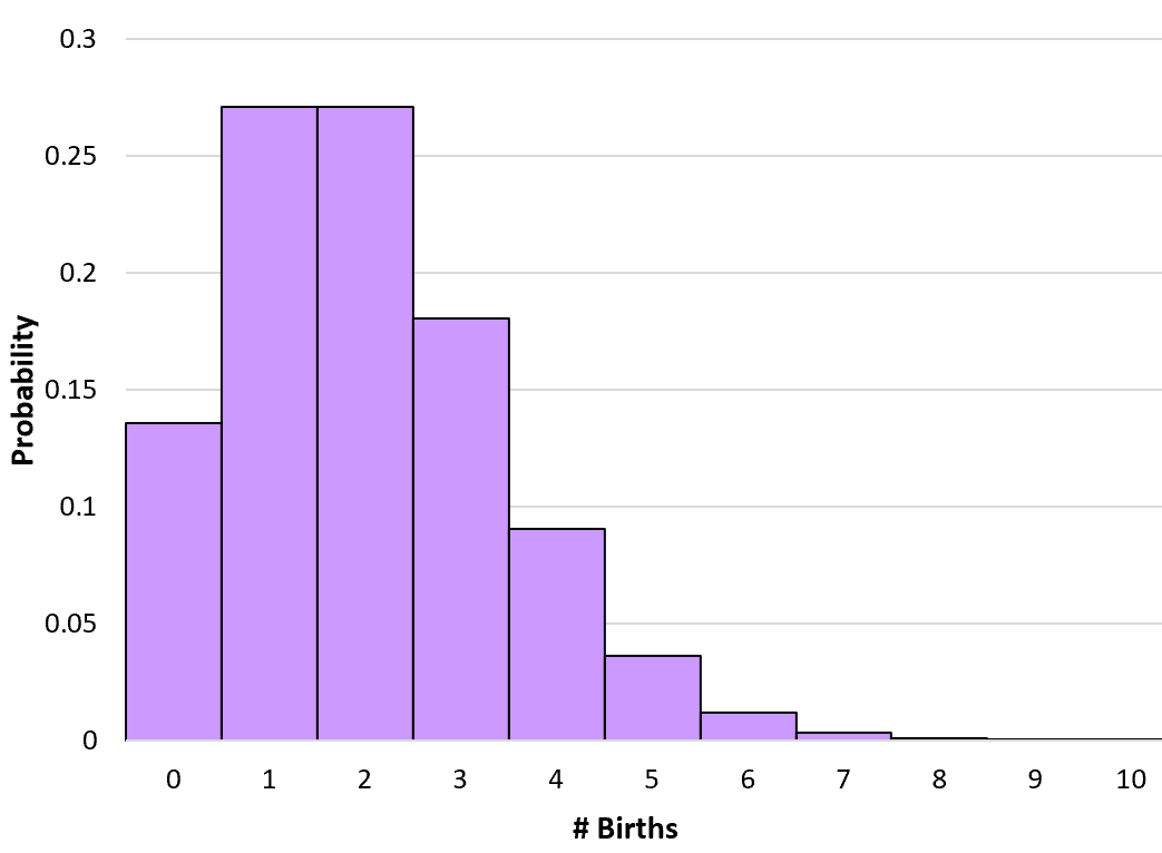
We often visualize probability mass functions with bar charts.
For example, the following bar chart shows the probabilities associated with the number of births per hour for the Poisson distribution described in the previous example:

Note that the number of births could extend to infinity, but the probabilities become so low after 10 that we can’t even see them on a bar chart.
Properties of a PMF
A probability mass function has the following properties:
1. All probabilities are positive in the support. For example, the probability that a dice lands between 1 and 6 is positive, while the probability of all other outcomes is equal to zero.
2. All outcomes have a probability between 0 and 1. For example, the probability that a dice lands between 1 and 6 is 1/6, or 0.1666666 for each outcome.
3. The sum of all probabilities must add up to 1. For example, the sum of probabilities that a dice lands on a certain number is 1/6 + 1/6 + 1/6 + 1/6 + 1/6 + 1/6 = 1.
Additional Resources
What Are Random Variables?
CDF vs. PDF: What’s the Difference?
An Introduction to the Binomial Distribution
An Introduction to the Poisson Distribution
