How to Perform Polynomial Regression in SAS

---

The most common type of regression analysis is simple linear regression, which is used when a predictor variable and a response variable have a linear relationship.

However, sometimes the relationship between a predictor variable and a response variable is nonlinear. 

In these cases it makes sense to use polynomial regression, which can account for the nonlinear relationship between the variables.

The following example shows how to perform polynomial regression in SAS.

Example: Polynomial Regression in SAS

Suppose we have the following dataset in SAS:

/*create dataset*/
data my_data;
    input x y;
    datalines;
2 18
4 14
4 16
5 17
6 18
7 23
7 25
8 28
9 32
12 29
;
run;

/*view dataset*/
proc print data=my_data;

Now suppose we create a scatter plot to visualize the relationship between the variables x and y in the dataset:

/*create scatter plot of x vs. y*/
proc sgplot data=my_data;
    scatter x=x y=y;
run;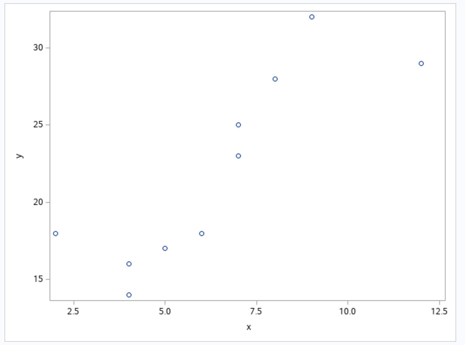

From the plot we can see that the relationship between x and y appears to be cubic.

Thus, we can define two new predictor variables in our dataset (x² and x³) and then use proc reg to fit a polynomial regression model using these predictor variables:

/*create dataset with new predictor variables*/
data my_data;
    input x y;
    x2 = x**2;
    x3 = x**3;
    datalines;
2 18
4 14
4 16
5 17
6 18
7 23
7 25
8 28
9 32
12 29
;
run;

/*fit polynomial regression model*/
proc reg data=my_data;
    model y = x x2 x3;
run;

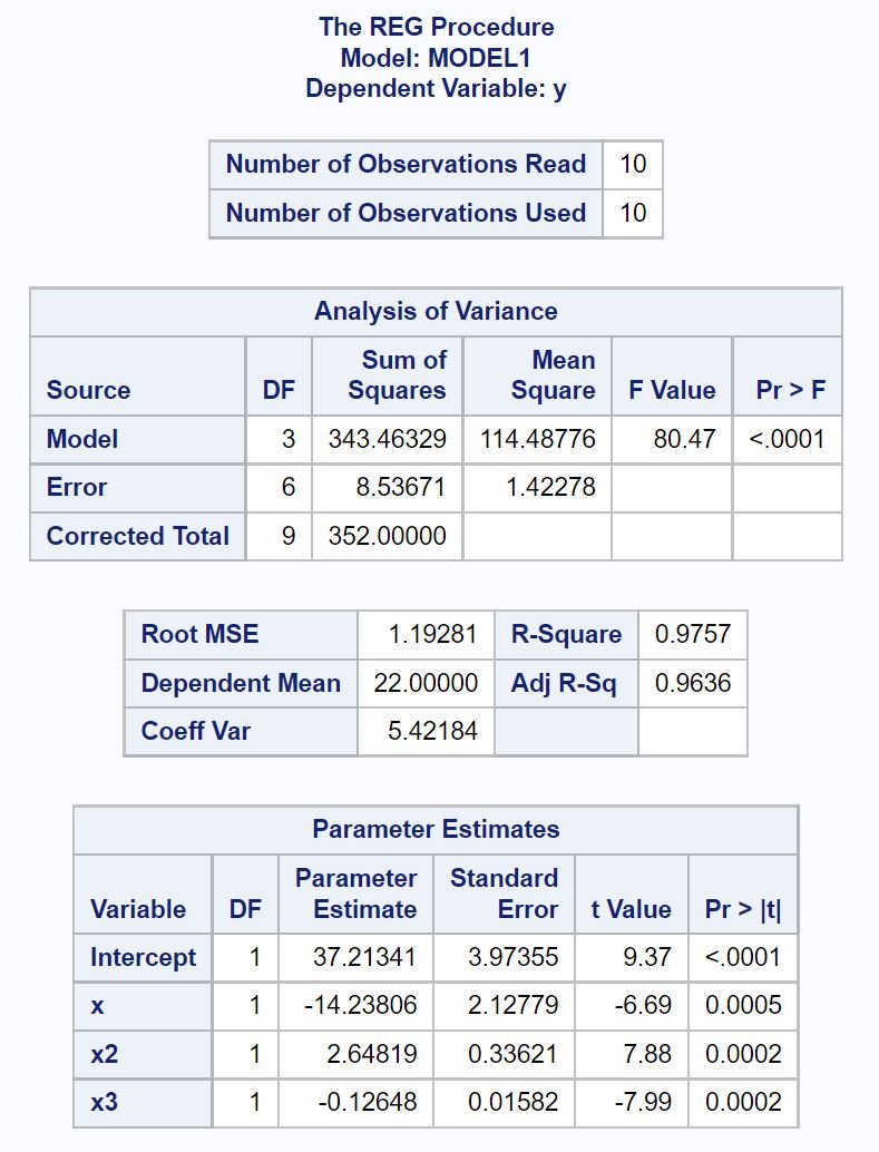
From the Parameter Estimates table we can find the coefficient estimates and write our fitted polynomial regression equation as:

y = 37.213 – 14.238x + 2.648x² – 0.126x³

This equation can be used to find the expected value for the response variable based on a given value for the predictor variable.

For example if x has a value of 4 then y is expected to have a value of 14.565:

y = 37.213 – 14.238(4) + 2.648(4)² – 0.126(4)³ = 14.565

We can also see the polynomial regression model has an adjusted R-squared value of 0.9636, which is extremely close to one and tells us that the model does an excellent job of fitting the dataset.

Related: How to Interpret Adjusted R-Squared (With Examples)

Additional Resources

The following tutorials explain how to perform other common tasks in SAS:

How to Perform Simple Linear Regression in SAS
How to Perform Multiple Linear Regression in SAS
How to Perform Quantile Regression in SAS