How to Perform Quadratic Regression in SPSS

---

When two variables have a linear relationship, you can often use simple linear regression to quantify their relationship.

However, simple linear regression doesn’t work well when two variables have a non-linear relationship. In these cases, you can try using quadratic regression. 

This tutorial explains how to perform quadratic regression in SPSS.

Example: Quadratic Regression in SPSS

Suppose we are interested in understanding the relationship between number of hours worked and happiness. We have the following data on the number of hours worked per week and the reported happiness level (on a scale of 0-100) for 16 different people:

Use the following steps to perform a quadratic regression in SPSS.

Step 1: Visualize the data.

Before we perform quadratic regression, let’s make a scatterplot to visualize the relationship between hours worked and happiness to verify that the two variables actually have a quadratic relationship.

Click the Graphs tab, then Chart Builder:

In the new window that pops up, choose Scatter/Dot in the Choose from list. Then drag the chart titled Simple Scatter into the main editing window. Drag the variable hours onto the x-axis and happiness onto the y-axis. Then click OK.

The following scatterplot will appear:

We can clearly see that a non-linear relationship exists between hours worked and happiness. This tells us that quadratic regression is an appropriate technique to use in this situation.

Step 2: Create a new variable.

Before we can perform quadratic regression, we need to create a predictor variable for hours².

Click the Transform tab, then Compute variable:

In the new window that pops up, name the target variable hours2 and define it as hours*hours:

Once you click OK, the variable hours2 will appear in a new column:

Step 3: Perform quadratic regression.

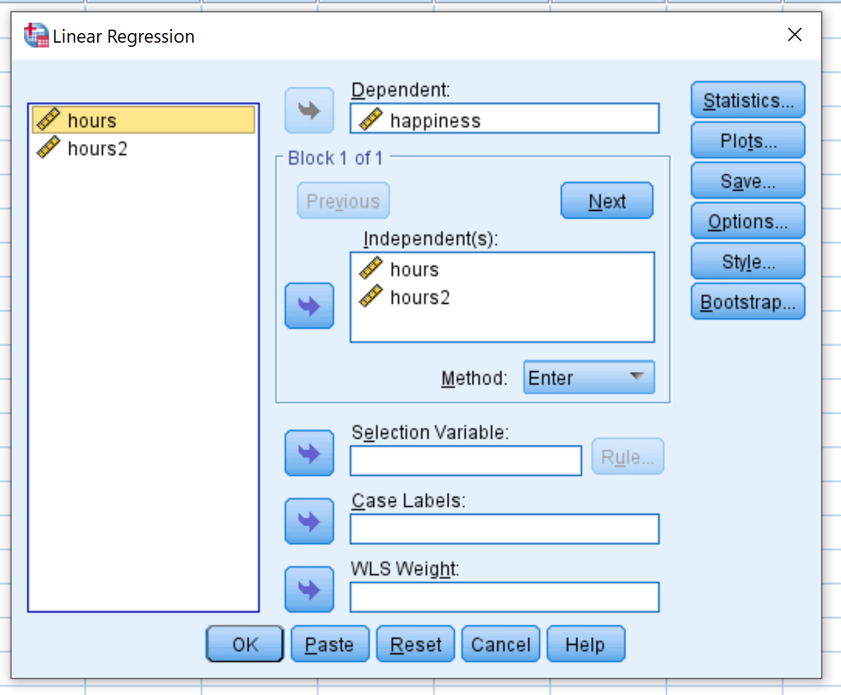
Next, we will perform quadratic regression. Click on the Analyze tab, then Regression, then Linear:

In the new window that pops up, drag happiness into the boxed labeled Dependent. Drag hours and hours2 into the box labeled Independent(s). Then click OK.

Step 4: Interpret the results.

Once you click OK, the results of the quadratic regression will appear in a new window.

The first table we’re interested in is titled Model Summary:

Here is how to interpret the most relevant numbers in this table:

• R Square: This is the proportion of the variance in the response variable that can be explained by the explanatory variables. In this example, 90.9% of the variation in happiness can be explained by the variables hours and hours².
• Std. Error of the Estimate: The standard error is the average distance that the observed values fall from the regression line. In this example, the observed values fall an average of 9.519 units from the regression line.

The next table we’re interested in is titled ANOVA:

Here is how to interpret the most relevant numbers in this table:

• F: This is the overall F statistic for the regression model, calculated as Mean Square Regression / Mean Square Residual.
• Sig: This is the p-value associated with the overall F statistic. It tells us whether or not the regression model as a whole is statistically significant. In this case the p-value is equal to 0.000, which indicates that the explanatory variables hours and hours² combined have a statistically significant association with exam score.

The next table we’re interested in is titled Coefficients:

We can use the values in the column Unstandardized B to form the estimated regression equation for this dataset:

Estimated happiness level = -30.253 + 7.173*(hours) – .107*(hours²)

We can use this equation to find the estimated happiness level for an individual based on the number of hours they work per week. For example, an individual that works 60 hours per week is expected to have a happiness level of 14.97:

Estimated happiness level = -30.253 + 7.173*(60) – .107*(60²) = 14.97.

Conversely, an individual that works 30 hours perk week is predicted to have a happiness level of 88.65:

Estimated happiness level = -30.253 + 7.173*(30) – .107*(30²) = 88.65.

Step 5: Report the results.

Lastly, we want to report the results of our quadratic regression. Here is an example of how to do so:

A quadratic regression was performed to quantify the relationship between the number of hours worked by an individual and their corresponding happiness level (measured from 0 to 100). A sample of 16 individuals was used in the analysis.

 

Results showed that there was a statistically significant relationship between the explanatory variables hours and hours² and the response variable happiness (F(2, 13) = 65.095, p

 

Combined, these two explanatory variables accounted for 90.9% of variability in happiness. 

 

The regression equation was found to be:

 

Estimated happiness level  = -30.253 + 7.173(hours) – .107(hours²)