Linear regression is a method we can use to understand the relationship between one or more predictor variables and a response variable.
Typically when we perform linear regression, we’re interested in estimating the mean value of the response variable.
However, we could instead use a method known as quantile regression to estimate any quantile or percentile value of the response value such as the 70th percentile, 90th percentile, 98th percentile, etc.
To perform quantile regression in R we can use the rq() function from the quantreg package, which uses the following syntax:
library(quantreg)

model 0.5)
where:
- y: The response variable
- x: The predictor variable(s)
- data: The name of the dataset
- tau: The percentile to find. The default is the median (tau = 0.5) but you can set this to any number between 0 and 1.
This tutorial provides a step-by-step example of how to use this function to perform quantile regression in R.
Step 1: Enter the Data
For this example we’ll create a dataset that contains the hours studied and the exam score received for 100 different students at some university:
#make this example reproducible
set.seed(0)

#create data frame
hours #view first six rows
head(df)

     hours    score
1 9.070275 79.22682
2 3.389578 66.20457
3 4.349115 73.47623
4 6.155680 70.10823
5 9.173870 78.12119
6 2.815137 65.94716
Step 2: Perform Quantile Regression
Next, we’ll fit a quantile regression model using hours studied as the predictor variable and exam score as the response variable.
We’ll use the model to predict the expected 90th percentile of exam scores based on the number of hours studied:
library(quantreg)

#fit model
model 0.9)

#view summary of model
summary(model)

Call: rq(formula = score ~ hours, tau = 0.9, data = df)

tau: [1] 0.9

Coefficients:
            coefficients lower bd upper bd
(Intercept) 60.25185     59.27193 62.56459
hours        2.43746      1.98094  2.76989
From the output, we can see the estimated regression equation:
90th percentile of exam score = 60.25 + 2.437*(hours)
For example, the 90th percentile of scores for all students who study 8 hours is expected to be 79.75:
90th percentile of exam score = 60.25 + 2.437*(8) = 79.75.
The output also displays the upper and lower confidence limits for the intercept and the predictor variable hours.
Step 3: Visualize the Results
We can also visualize the results of the regression by creating a scatterplot with the fitted quantile regression equation overlaid on the plot:
library(ggplot2)

#create scatterplot with quantile regression line
ggplot(df, aes(hours,score)) +
  geom_point() +
  geom_abline(intercept=coef(model)[1], slope=coef(model)[2])

Unlike a traditional linear regression line, notice that this fitted line doesn’t go through the heart of the data. Instead, it goes through the estimated 90th percentile at each level of the predictor variable.
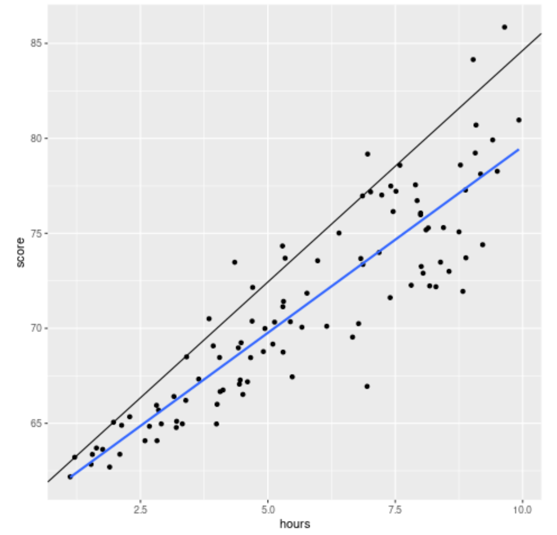
We can view the difference between the fitted quantile regression equation and the simple linear regression equation by adding the geom_smooth() argument:
library(ggplot2)

#create scatterplot with quantile regression line and simple linear regression line
ggplot(df, aes(hours,score)) +
  geom_point() +
  geom_abline(intercept=coef(model)[1], slope=coef(model)[2]) +
  geom_smooth(method="lm", se=F)

The black line displays the fitted quantile regression line for the 90th percentile and the blue line displays the simple linear regression line, which estimates the mean value for the response variable.
As expected, the simple linear regression line goes straight through the data and shows us the mean estimated value of exam scores at each level of hours.
Additional Resources
The following tutorials explain how to perform other common tasks in R:
How to Perform Simple Linear Regression in R
How to Perform Multiple Linear Regression in R
How to Perform Quadratic Regression in R
