In this lesson you can learn how to freeze panes and how to split spreadseet.
You can use it, when you want to work in Excel with big data bases in your worksheet easier. You can do something like that:
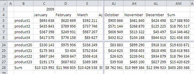
Let's see, how to do it.
You have quite a large table that does not fit in the Excel. For this reason, you do not see headers and it is hard you work. The table in this form is completely unreadable, but you can easily fix it.
Freeze Panes
Freezing Panes is that when scrolling the window of the table is in the same place. For example, you can block top row or first column of the table so to still have them visible. You know then, which means the data cell. In the picture you can't to see that. I will teach you to freeze header row and first column at the same time. Select the cell that is under the top row (row 4) and the right of the first column (column B). Typically, this is cell B2 but I did it C% for better understanding.
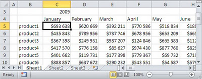
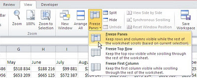
Go to the ribbon. Choose View - Freeze Pane
Worksheet is frozen. Now, moving a table, row and column header will always be visible.
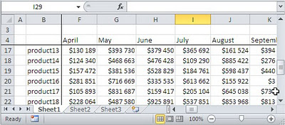
Note: Keyboard Shortcut for Freeze Panes is Alt + W + F + F
Worksheet Split
Another situation is when you haven't got enough space in the Worksheet. For example you need to have access to different parts of the sheet simultaneously. To avoid continuous scrolling, let's split it. In order to split the window in Excel, first select one of the cells. Then go to the ribbon according to the path: View - Split
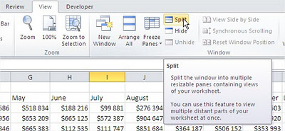
The screen was divided into four parts, which you can scroll independently! This is a great convenience in working with large data sheets.

Note: Keyboard Shortcut for Freeze Panes is Alt + W + S
Further reading:
Text to Columns
Grid
How to compare columns to find duplicates?