How to remove duplicates in Excel
In this digital era, duplicate values in your datasheet are common, but it can be a big problem. It can induce substantial error and overestimate your outcomes. With the help of Excel’s Eliminate Duplicate feature, you can instantly find and remove duplicates form rows or columns. It is a significant feature of Excel, especially when dealing with the huge data sets in which various people put the values in the data sets.
If you want to remove duplicates in Excel, form your data, you can do this easily in Excel. Read on this tutorial to know how to find and remove duplicate values from your data in Excel.
Method 1
Removing duplicates
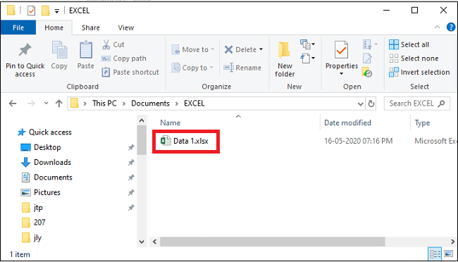
Double click your Excel Document:
Open your computer device and double click your Excel Document, you will be navigated to the spreadsheet in Excel.
It allows you to open an existing document from the “Recent” option of the open tab.
Select the data:
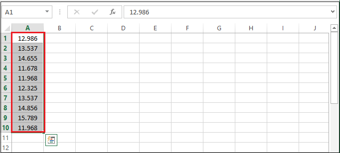
From the Excel spreadsheet, you need to select the data. For the data selection, click the top entry of the data and hold down the Shift key and click on the bottom entry.
If you are going to select multiple columns simultaneously, you need to click the top-left entry of data, then click the bottom right entry of data while holding down the Shift key.
Click the Data tab:
Once you select the data from the spreadsheet, you need to click on the Data tab located at the top of the Excel window.

Click Remove Duplicates:
If you click on the Data tab, a drop-down menu will appear with a list of options, where you need to click the “Remove Duplicates” option. This option is the “Data tools” section of the Data tab located at the top of the Excel window.

Ensure that each column you want to edit is selected:
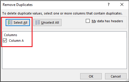
If you click on the Remove Duplicates option, a pop-up will appear where you need to ensure the first thing that you have selected each column you want to edit in the spreadsheet. On the spreadsheet, you will find various column names, for example, Column A, Column B, and so on next to the checkboxes, cling checkboxes will lead to de-select the column, so you need to be careful.
In the Excel spreadsheet, all columns next to the one you choose will be listed and checked by default.
It allows you to click and Select All to select all of the columns listed here.
Click Ok when prompted:
If you click on the ok tab located at the bottom right corner of the Remove duplicates windows, a pop-up will appear, where you need to click on the “Ok” tab, doing so will remove any duplicates from your Excel sheet.
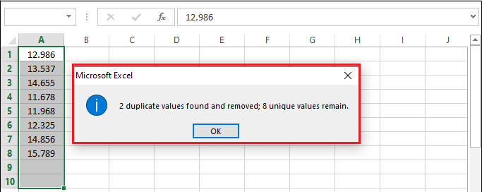
If no duplicates are shown when you know there are duplicates, you need to try and select one column at a time.
Method 2
Highlighting Duplicates
Double click your Excel document:
Open your computer and double click your Excel document with whom you wish to edit. If you click on the document, it will open the spreadsheet in Excel. It enables you to check it for cells consisting of duplicate data values using the Conditional Formatting feature of Excel. If you wish to look for duplicates, but you don’t want to remove them by default, this is a good option for you to doing so.
It also enables you to open an existing document for the “Recent” section of the Open tab.

Click the top-left cell in your data group:
Once you select the document whom you wish to edit, you need to click the top-left cell on the data group; doing so will select it.
Here, you need to exclude headers, for example, Day, Date, Time, etc. form your selection list.
If you are going to choose one row, you need to click the left-most entry from the data group.
If you are going to select one column, you need to click on the rightmost entry from the data group.
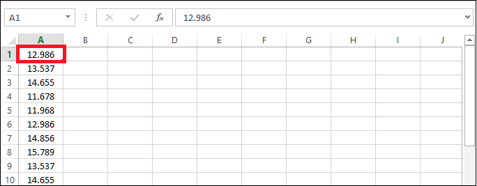
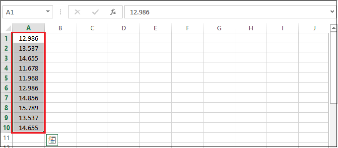
Hold on the shift key and click the bottom right cell:
After now, you need to hold on the Shift key and click the bottom right cell. It will help you to select any data between the top-left corner and the bottom right corner of the data group.
If you are going to select a single row, you need to click the rightmost cell with value in it.
If you are going to select a single column, you need to click the bottom-most entry with value in it.
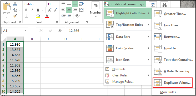
Click Conditional formatting:
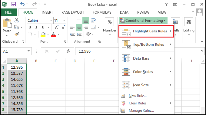
You will find the conditional formatting option in the “Styles” section of the Home page. If you click on “Conditional Formatting,” a drop-down menu will appear.
You may have to click the “Home” tab located near the top of the Excel page to see this option.

Choose Highlight cells rules:
From the drop-down menu, you need to select the “Highlight cells rules.” Once you click on highlight cell rules, a pop-up will appear.
Click Duplicates value:
From the pop-up menu. You need to select “Duplicates Values” located at the bottom of the menu, doing so will select all duplicates value.
